Step 3: Perform fit¶

As explained in the previous step, an IntensityTF object behaves just like a mathematical function that takes a set of data points as an argument and returns a list of intensities (real numbers). At this stage, we want to optimize the parameters of the intensity model, so that it matches the distribution of our data sample. This is what we call ‘performing a fit’.

Note

We first load the relevant data from the previous steps.

import numpy as np
from expertsystem import io

from tensorwaves.physics.helicity_formalism.amplitude import IntensityBuilder
from tensorwaves.physics.helicity_formalism.kinematics import HelicityKinematics

model = io.load("amplitude_model_helicity.yml")
kinematics = HelicityKinematics.from_model(model)
data_sample = np.load("data_sample.npy")
phsp_sample = np.load("phsp_sample.npy")
intensity_builder = IntensityBuilder(model.particles, kinematics)
intensity = intensity_builder.create_intensity(model)
phsp_set = kinematics.convert(phsp_sample)
data_set = kinematics.convert(data_sample)

3.1 Define estimator¶

To perform a fit, you need to define an estimator. An estimator is a measure for the discrepancy between the intensity model and the data distribution to which you fit. In PWA, we usually use an unbinned negative log likelihood estimator, which can be created as follows with the tensorwaves.estimator module.

Generally the intensity model is not normalized, but a log likelihood estimator requires a normalized function. This is where the phase space dataset comes into play! The intensity is separately evaluated with the phase space dataset and the normalization is achieved in this way. It is a required argument! Note that if you want to correct for the efficiency of the detector, a detector-reconstructed phase space dataset should be inserted here.

from tensorwaves.estimator import UnbinnedNLL

estimator = UnbinnedNLL(intensity, data_set, phsp_set)

The parameters that the UnbinnedNLL carries, have been taken from the IntensityTF object and you’ll recognize them from the YAML recipe file that we created in Step 1:

estimator.parameters

{'MesonRadius_J/psi(1S)': 1.0,
 'Magnitude_J/psi(1S)_to_f(0)(500)_0+gamma_1;f(0)(500)_to_pi0_0+pi0_0;': 1.0,
 'Phase_J/psi(1S)_to_f(0)(500)_0+gamma_1;f(0)(500)_to_pi0_0+pi0_0;': 0.0,
 'Magnitude_J/psi(1S)_to_f(0)(1500)_0+gamma_1;f(0)(1500)_to_pi0_0+pi0_0;': 1.0,
 'Phase_J/psi(1S)_to_f(0)(1500)_0+gamma_1;f(0)(1500)_to_pi0_0+pi0_0;': 0.0,
 'Magnitude_J/psi(1S)_to_f(0)(1710)_0+gamma_1;f(0)(1710)_to_pi0_0+pi0_0;': 1.0,
 'Phase_J/psi(1S)_to_f(0)(1710)_0+gamma_1;f(0)(1710)_to_pi0_0+pi0_0;': 0.0,
 'Magnitude_J/psi(1S)_to_f(0)(1370)_0+gamma_1;f(0)(1370)_to_pi0_0+pi0_0;': 1.0,
 'Phase_J/psi(1S)_to_f(0)(1370)_0+gamma_1;f(0)(1370)_to_pi0_0+pi0_0;': 0.0,
 'Magnitude_J/psi(1S)_to_f(0)(980)_0+gamma_1;f(0)(980)_to_pi0_0+pi0_0;': 1.0,
 'Phase_J/psi(1S)_to_f(0)(980)_0+gamma_1;f(0)(980)_to_pi0_0+pi0_0;': 0.0,
 'Position_f(0)(1500)': 1.506,
 'Width_f(0)(1500)': 0.112,
 'MesonRadius_f(0)(1500)': 1.0,
 'Position_f(0)(500)': 0.475,
 'Width_f(0)(500)': 0.55,
 'MesonRadius_f(0)(500)': 1.0,
 'Position_f(0)(1710)': 1.704,
 'Width_f(0)(1710)': 0.123,
 'MesonRadius_f(0)(1710)': 1.0,
 'Position_f(0)(980)': 0.99,
 'Width_f(0)(980)': 0.06,
 'MesonRadius_f(0)(980)': 1.0,
 'Position_f(0)(1370)': 1.35,
 'Width_f(0)(1370)': 0.35,
 'MesonRadius_f(0)(1370)': 1.0,
 'Position_J/psi(1S)': 3.0969,
 'Width_J/psi(1S)': 9.29e-05}

3.2 Optimize the intensity model¶

Now it’s time to perform the fit! This is the part where the TensorFlow backend comes into play. For this reason, we suppress a few warnings:

import tensorflow as tf

tf.get_logger().setLevel("ERROR")

Starting the fit itself is quite simple: just create an optimizer instance of your choice, here Minuit2, and call its optimize method to start the fitting process. Notice that the optimize method requires a second argument. This is a mapping of parameter names that you want to fit to their initial values.

Let’s first select a few of the parameters that we saw in Step 3.1 and feed them to the optimizer to run the fit. Notice that we modify the parameters slightly to make the fit more interesting (we are running using a data sample that was generated with this very amplitude model after all).

initial_parameters = {
    "Phase_J/psi(1S)_to_f(0)(1500)_0+gamma_1;f(0)(1500)_to_pi0_0+pi0_0;": 0.0,
    "Width_f(0)(500)": 0.3,
    "Width_f(0)(980)": 0.1,
    "Position_f(0)(1710)": 1.75,
    "Width_f(0)(1710)": 0.2,
}

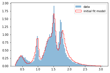
Recall that an IntensityTF object is really just a Function that computes the intensity for a certain dataset. This can be seen now nicely when we use these intensities as weights on the phase space sample and plot it together with the original dataset. Here, we look at the invariant mass distribution projection of the final states 3 and 4, which, as we saw before, are the final state particles \(\pi^0,\pi^0\).

Don’t forget to use update_parameters first!

import matplotlib.pyplot as plt
import numpy as np


def compare_model(
    variable_name, data_set, phsp_set, intensity_model, transform=lambda p: p, bins=100
):
    data = transform(data_set[variable_name])
    phsp = transform(phsp_set[variable_name])
    intensities = intensity_model(phsp_set)
    plt.hist(data, bins=bins, alpha=0.5, label="data", density=True)
    plt.hist(
        phsp,
        weights=intensities,
        bins=bins,
        histtype="step",
        color="red",
        label="initial fit model",
        density=True,
    )
    plt.legend()

intensity.update_parameters(initial_parameters)
compare_model("mSq_3+4", data_set, phsp_set, intensity, np.sqrt)

Finally, we create an Optimizer to optimize the model (which is embedded in the Estimator. Only the parameters that are given to the optimize method are optimized.

Here, we choose to use Minuit2, which is the most common optimizer choice in high-energy physics. Notice that the Minuit2 class allows one to list callbacks. These are called during the optimize() method. Here, we use CallbackList to ‘stack’ several callbacks together.

To define your own callback, create a class that inherits from the Callback class and feed it to the Minuit2 constructor.

from tensorwaves.optimizer.callbacks import (
    CallbackList,
    CSVSummary,
    TFSummary,
    YAMLSummary,
)
from tensorwaves.optimizer.minuit import Minuit2

minuit2 = Minuit2(
    callback=CallbackList(
        [
            TFSummary(),
            YAMLSummary("current_fit_result.yaml"),
            CSVSummary("fit_traceback.csv", step_size=2),
        ]
    )
)
result = minuit2.optimize(estimator, initial_parameters)
result

{'parameter_values': {'Phase_J/psi(1S)_to_f(0)(1500)_0+gamma_1;f(0)(1500)_to_pi0_0+pi0_0;': 0.010969293771242894,
  'Width_f(0)(500)': 0.555914748706843,
  'Width_f(0)(980)': 0.05987333350304519,
  'Position_f(0)(1710)': 1.7028547245990788,
  'Width_f(0)(1710)': 0.12239115415507927},
 'parameter_errors': {'Phase_J/psi(1S)_to_f(0)(1500)_0+gamma_1;f(0)(1500)_to_pi0_0+pi0_0;': 0.022475163245250743,
  'Width_f(0)(500)': 0.01387083421811444,
  'Width_f(0)(980)': 0.0017700174418181264,
  'Position_f(0)(1710)': 0.0011982413597589332,
  'Width_f(0)(1710)': 0.0034941216494044722},
 'log_likelihood': -13426.004198736486,
 'function_calls': 176,
 'execution_time': 157.54964423179626}

Computation time ― around a minute in this case

The computation time depends on the complexity of the model, number of data events, the size of the phase space sample, and the number of free parameters. This model is rather small and has but a few free parameters, so the optimization shouldn’t take more than a few minutes.

As can be seen, the values of the optimized parameters in the result are again comparable to the original values we saw in 3.1 Define estimator:

optimized_parameters = result["parameter_values"]
optimized_parameters

{'Phase_J/psi(1S)_to_f(0)(1500)_0+gamma_1;f(0)(1500)_to_pi0_0+pi0_0;': 0.010969293771242894,
 'Width_f(0)(500)': 0.555914748706843,
 'Width_f(0)(980)': 0.05987333350304519,
 'Position_f(0)(1710)': 1.7028547245990788,
 'Width_f(0)(1710)': 0.12239115415507927}

3.3 Export and import¶

In 3.2 Optimize the intensity model, we initialized Minuit2 with some callbacks that are Loadable. Such callback classes offer the possibility to Loadable.load_latest_parameters(), so you can pick up the optimize process in case it crashes or if you pause it. Loading the latest parameters goes as follows:

latest_parameters = YAMLSummary.load_latest_parameters("current_fit_result.yaml")
latest_parameters

{'Phase_J/psi(1S)_to_f(0)(1500)_0+gamma_1;f(0)(1500)_to_pi0_0+pi0_0;': 0.012496387788803603,
 'Width_f(0)(500)': 0.555914748706843,
 'Width_f(0)(980)': 0.05987333350304519,
 'Position_f(0)(1710)': 1.7028547245990788,
 'Width_f(0)(1710)': 0.12264377011041581}

To restart the fit with the latest parameters, simply rerun as before.

minuit2 = Minuit2()
minuit2.optimize(estimator, latest_parameters)

{'parameter_values': {'Phase_J/psi(1S)_to_f(0)(1500)_0+gamma_1;f(0)(1500)_to_pi0_0+pi0_0;': 0.010970542137489854,
  'Width_f(0)(500)': 0.5559040414550535,
  'Width_f(0)(980)': 0.05987107480308382,
  'Position_f(0)(1710)': 1.7028548023543402,
  'Width_f(0)(1710)': 0.12239320337468709},
 'parameter_errors': {'Phase_J/psi(1S)_to_f(0)(1500)_0+gamma_1;f(0)(1500)_to_pi0_0+pi0_0;': 0.022475339801068445,
  'Width_f(0)(500)': 0.013870447926612926,
  'Width_f(0)(980)': 0.001769926627552895,
  'Position_f(0)(1710)': 0.0011982498399639291,
  'Width_f(0)(1710)': 0.0034942212183679045},
 'log_likelihood': -13426.004198272767,
 'function_calls': 96,
 'execution_time': 92.15698432922363}

Lo and behold: the parameters were already optimized, so the fit converged faster!

3.4 Visualize¶

Plot optimized model¶

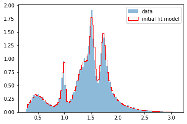
Using the same method as above, we renew the parameters of the IntensityTF and plot it again over the data distribution.

intensity.update_parameters(latest_parameters)
compare_model("mSq_3+4", data_set, phsp_set, intensity, np.sqrt)

Analyze optimization process¶

Note that in Step 3.2, we initialized Minuit2 with a TFSummary callback as well. Its output files provide a nice, interactive representation of the fit process and can be viewed with TensorBoard as follows:

Terminal

tensorboard --logdir logs

Python

import tensorboard as tb

tb.notebook.list()  # View open TensorBoard instances
tb.notebook.start(args_string="--logdir logs")

See more info here

Jupyter notebook

%load_ext tensorboard
%tensorboard --logdir logs

See more info here

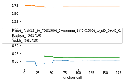
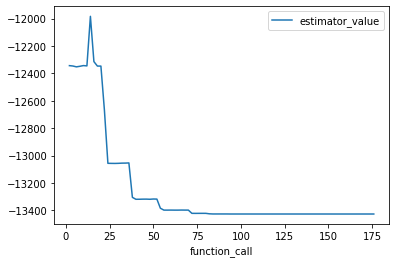
An alternative would be to use the output of the CSVSummary callback. Here’s an example:

import pandas as pd

fit_traceback = pd.read_csv("fit_traceback.csv")

fit_traceback.plot("function_call", "estimator_value");

fit_traceback.plot(
    "function_call",
    [
        "Phase_J/psi(1S)_to_f(0)(1500)_0+gamma_1;f(0)(1500)_to_pi0_0+pi0_0;",
        "Position_f(0)(1710)",
        "Width_f(0)(1710)",
    ],
);

TensorWaves