Step 2: Generate data samples
In this section, we will use the AmplitudeModel that we created with the expert system in the previous step to generate a data sample via hit & miss Monte Carlo. We do this with the data.generate module.
First, we load() an AmplitudeModel that was created in the previous step:
from expertsystem import io

model = io.load("amplitude_model_helicity.yml")
2.1 Define kinematics of the particle reaction
An AmplitudeModel defines the kinematics, the particles involved in the reaction, the dynamics used for the model on which to perform the eventual optimization, etc.
from tensorwaves.physics.helicity_formalism.kinematics import (
    HelicityKinematics,
)

kin = HelicityKinematics.from_model(model)
print("Initial state mass:", kin.reaction_kinematics_info.initial_state_masses)
print("Final state masses:", kin.reaction_kinematics_info.final_state_masses)
print("Involved particles:", model.particles.names)
Initial state mass: [3.0969]
Final state masses: [0.0, 0.1349768, 0.1349768]
Involved particles: {'f(0)(1370)', 'f(0)(980)', 'gamma', 'f(0)(500)', 'f(0)(1500)', 'f(0)(1710)', 'pi0', 'J/psi(1S)'}
A Kinematics object defines the kinematics of the particle reaction we are studying. From the final state masses listed here, we can see we are dealing with the reaction \(J/\psi \to \gamma\pi^0\pi^0\).
2.2 Generate phase space sample
Kinematics define the constraints of the phase space. As such, we have enough information to generate a phase-space sample for this particle reaction. We do this with the generate_phsp() function. By default, this function uses TFPhaseSpaceGenerator as a, well… phase-space generator (using tensorflow in the back-end) and generates random numbers with TFUniformRealNumberGenerator. You can specify this with the arguments of generate_phsp() function.
from tensorwaves.data.generate import generate_phsp

phsp_sample = generate_phsp(300_000, kin)
phsp_sample.shape
(3, 300000, 4)
As you can see, the phase-space sample is a three-dimensional array: 300.000 events of four-momentum tuples for three particles.
2.3 Generate intensity-based sample
‘Data samples’ are more complicated than phase space samples in that they represent the intensity profile resulting from a reaction. You therefore need an IntensityTF object (or, more generally, a Function instance) and a phase space over which to generate that intensity distribution. We call such a data sample an intensity-based sample.
An intensity-based sample is generated with the function generate_data(). Its usage is similar to generate_phsp(), but now you have to give an IntensityTF in addition to the Kinematics object. An IntensityTF object can be created with the IntensityBuilder class:
from tensorwaves.physics.helicity_formalism.amplitude import IntensityBuilder

builder = IntensityBuilder(model.particles, kin)
intensity = builder.create_intensity(model)
That’s it, now we have enough info to create an intensity-based data sample. Notice how the structure is the sample as the phase-space sample we saw before:
from tensorwaves.data.generate import generate_data

data_sample = generate_data(30_000, kin, intensity)
data_sample.shape
WARNING:tensorflow:5 out of the last 5 calls to <function polar at 0x7fe489d23a60> triggered tf.function retracing. Tracing is expensive and the excessive number of tracings could be due to (1) creating @tf.function repeatedly in a loop, (2) passing tensors with different shapes, (3) passing Python objects instead of tensors. For (1), please define your @tf.function outside of the loop. For (2), @tf.function has experimental_relax_shapes=True option that relaxes argument shapes that can avoid unnecessary retracing. For (3), please refer to https://www.tensorflow.org/guide/function#controlling_retracing and https://www.tensorflow.org/api_docs/python/tf/function for more details.
WARNING:tensorflow:5 out of the last 5 calls to <function relativistic_breit_wigner at 0x7fe489ca4280> triggered tf.function retracing. Tracing is expensive and the excessive number of tracings could be due to (1) creating @tf.function repeatedly in a loop, (2) passing tensors with different shapes, (3) passing Python objects instead of tensors. For (1), please define your @tf.function outside of the loop. For (2), @tf.function has experimental_relax_shapes=True option that relaxes argument shapes that can avoid unnecessary retracing. For (3), please refer to https://www.tensorflow.org/guide/function#controlling_retracing and https://www.tensorflow.org/api_docs/python/tf/function for more details.
(3, 30000, 4)
2.4 Visualize kinematic variables
We now have a phase space sample and an intensity-based sample. Their data structure isn’t the most informative though: it’s just a collection of four-momentum tuples. However, we can use the Kinematics class to convert those four-momentum tuples to a data set of kinematic variables.
Now we can use the Kinematics.convert() method to convert the phase space and data samples of four-momentum tuples to kinematic variables.
phsp_set = kin.convert(phsp_sample)
data_set = kin.convert(data_sample)
list(data_set)
['mSq_0+1+2',
 'mSq_0',
 'mSq_1+2',
 'mSq_1',
 'mSq_2',
 'theta_0_1+2',
 'phi_0_1+2',
 'theta_1_2_vs_0',
 'phi_1_2_vs_0']
The data set is just a dict of kinematic variables (keys are the names, values is a list of computed values for each event). The numbers you see here are final state IDs as defined in the AmplitudeModel member of the AmplitudeModel:
for state_id, particle in model.kinematics.final_state.items():
    print(f"ID {state_id}:", particle.name)
ID 0: gamma
ID 1: pi0
ID 2: pi0
Available kinematic variables
By default, tensorwaves only generates invariant masses of the SubSystems that are of relevance to the decay problem. In this case, we only have resonances \(f_0 \to \pi^0\pi^0\). If you are interested in more invariant mass combinations, you can do so with the method HelicityKinematics.register_invariant_mass(), e.g.:
kin.register_invariant_mass([2, 4])
The data set is dict, which allows us to easily convert it to a pandas.DataFrame and plot its content in the form of a histogram:
import pandas as pd

data_frame = pd.DataFrame(data_set)
phsp_frame = pd.DataFrame(phsp_set)
data_frame
| mSq_0+1+2 | mSq_0 | mSq_1+2 | mSq_1 | mSq_2 | theta_0_1+2 | phi_0_1+2 | theta_1_2_vs_0 | phi_1_2_vs_0 | |
|---|---|---|---|---|---|---|---|---|---|
| 0 | 9.59079 | 0.0 | 2.826263 | 0.018219 | 0.018219 | 0.982891 | -1.064371 | 1.019814 | -0.232838 |
| 1 | 9.59079 | 0.0 | 2.024409 | 0.018219 | 0.018219 | 0.646141 | 3.033674 | 2.393947 | -1.145904 |
| 2 | 9.59079 | 0.0 | 2.285591 | 0.018219 | 0.018219 | 2.333099 | -2.601390 | 2.358989 | -1.262855 |
| 3 | 9.59079 | 0.0 | 2.594168 | 0.018219 | 0.018219 | 2.361440 | -0.298117 | 1.763919 | -2.061845 |
| 4 | 9.59079 | 0.0 | 4.210845 | 0.018219 | 0.018219 | 1.717906 | 2.466436 | 1.365530 | 3.013163 |
| ... | ... | ... | ... | ... | ... | ... | ... | ... | ... |
| 29995 | 9.59079 | 0.0 | 1.314746 | 0.018219 | 0.018219 | 0.828402 | 0.047314 | 0.658794 | 0.037909 |
| 29996 | 9.59079 | 0.0 | 1.046369 | 0.018219 | 0.018219 | 1.554316 | -1.757748 | 0.834168 | 0.777405 |
| 29997 | 9.59079 | 0.0 | 2.943730 | 0.018219 | 0.018219 | 2.532420 | 0.647544 | 1.175604 | -1.126166 |
| 29998 | 9.59079 | 0.0 | 3.127327 | 0.018219 | 0.018219 | 1.085332 | 0.194296 | 0.452027 | 2.309917 |
| 29999 | 9.59079 | 0.0 | 3.272490 | 0.018219 | 0.018219 | 1.844568 | 0.367536 | 2.680698 | 1.797123 |
30000 rows × 9 columns
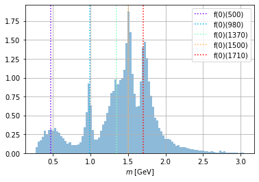
This also means that we can use all kinds of fancy plotting functionality of for instance matplotlib.pyplot to see what’s going on. Here’s an example:
import numpy as np
from matplotlib import cm

intermediate_states = sorted(
    (
        p
        for p in model.particles
        if p not in model.kinematics.final_state.values()
        and p not in model.kinematics.initial_state.values()
    ),
    key=lambda p: p.mass,
)

evenly_spaced_interval = np.linspace(0, 1, len(intermediate_states))
colors = [cm.rainbow(x) for x in evenly_spaced_interval]
import matplotlib.pyplot as plt

np.sqrt(data_frame["mSq_1+2"]).hist(bins=100, alpha=0.5, density=True)
plt.xlabel("$m$ [GeV]")
for i, p in enumerate(intermediate_states):
    plt.axvline(x=p.mass, linestyle="dotted", label=p.name, color=colors[i])
plt.legend();
2.5 Export data sets
tensorwaves currently has no export functionality for data samples. However, as we work with numpy.ndarray, it’s easy to just pickle these data samples with numpy.save():
import numpy as np

np.save("data_sample", data_sample)
np.save("phsp_sample", phsp_sample)
In the next step, we will illustrate how to ‘perform a fit’ with tensorwaves by optimizing the intensity model to these data samples.