Usage
TensorWaves is best suited for doing Partial Wave Analysis. First, the expertsystem determines which transitions are allowed from some initial state to a final state. It then formulates those transitions mathematically as an amplitude model. TensorWaves can then lambdify() this expression to some computational backend. Finally, TensorWaves ‘fits’ this model to some data sample. Optionally, this data sample can be generated from the model.
This page shows a brief overview of the complete workflow. More info about each step can be found under Step-by-step workflow.
Overview
Construct a model
See also
import expertsystem as es
import graphviz
import matplotlib.pyplot as plt
import pandas as pd
from expertsystem.amplitude.dynamics.builder import (
    create_relativistic_breit_wigner_with_ff,
)
from tensorwaves.data import generate_data, generate_phsp
from tensorwaves.data.transform import HelicityTransformer
from tensorwaves.estimator import UnbinnedNLL
from tensorwaves.model import LambdifiedFunction, SympyModel
from tensorwaves.optimizer.callbacks import CSVSummary
from tensorwaves.optimizer.minuit import Minuit2
result = es.generate_transitions(
    initial_state=("J/psi(1S)", [-1, +1]),
    final_state=["gamma", "pi0", "pi0"],
    allowed_intermediate_particles=["f(0)"],
    allowed_interaction_types=["strong", "EM"],
    formalism_type="canonical-helicity",
)
dot = es.io.asdot(result, collapse_graphs=True)
graphviz.Source(dot)

model_builder = es.amplitude.get_builder(result)
for name in result.get_intermediate_particles().names:
    model_builder.set_dynamics(name, create_relativistic_breit_wigner_with_ff)
model = model_builder.generate()
next(iter(model.components.values())).doit()
Generate data sample
See also
sympy_model = SympyModel(
    expression=model.expression,
    parameters=model.parameters,
)
intensity = LambdifiedFunction(sympy_model, backend="numpy")
data_converter = HelicityTransformer(model.adapter)
phsp_sample = generate_phsp(300_000, model.adapter.reaction_info)
data_sample = generate_data(
    30_000, model.adapter.reaction_info, data_converter, intensity
)
import numpy as np
from matplotlib import cm

reaction_info = model.adapter.reaction_info
intermediate_states = sorted(
    (
        p
        for p in model.particles
        if p not in reaction_info.final_state.values()
        and p not in reaction_info.initial_state.values()
    ),
    key=lambda p: p.mass,
)

evenly_spaced_interval = np.linspace(0, 1, len(intermediate_states))
colors = [cm.rainbow(x) for x in evenly_spaced_interval]


def indicate_masses():
    plt.xlabel("$m$ [GeV]")
    for i, p in enumerate(intermediate_states):
        plt.gca().axvline(
            x=p.mass, linestyle="dotted", label=p.name, color=colors[i]
        )
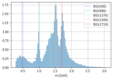
phsp_set = data_converter.transform(phsp_sample)
data_set = data_converter.transform(data_sample)
data_frame = pd.DataFrame(data_set.to_pandas())
data_frame["m_12"].hist(bins=100, alpha=0.5, density=True)
indicate_masses()
plt.legend();
Optimize the model
See also
import matplotlib.pyplot as plt
import numpy as np


def compare_model(
    variable_name,
    data_set,
    phsp_set,
    intensity_model,
    bins=150,
):
    data = data_set[variable_name]
    phsp = phsp_set[variable_name]
    intensities = intensity_model(phsp_set)
    plt.hist(data, bins=bins, alpha=0.5, label="data", density=True)
    plt.hist(
        phsp,
        weights=intensities,
        bins=bins,
        histtype="step",
        color="red",
        label="initial fit model",
        density=True,
    )
    indicate_masses()
    plt.legend()
estimator = UnbinnedNLL(
sympy_model,
data_set,
phsp_set,
backend="jax",
)
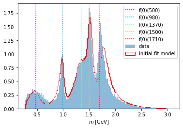
initial_parameters = {
"C[J/\\psi(1S) \\to f_{0}(1500)_{0} \\gamma_{+1};f_{0}(1500) \\to \\pi^{0}_{0} \\pi^{0}_{0}]": 1.0
+ 0.0j,
"Gamma_f(0)(500)": 0.3,
"Gamma_f(0)(980)": 0.1,
"m_f(0)(1710)": 1.75,
"Gamma_f(0)(1710)": 0.2,
}
intensity.update_parameters(initial_parameters)
compare_model("m_12", data_set, phsp_set, intensity)
print("Number of free parameters:", len(initial_parameters))
Number of free parameters: 5
callback = CSVSummary("traceback.csv", step_size=1)
minuit2 = Minuit2(callback)
fit_result = minuit2.optimize(estimator, initial_parameters)
fit_result
{'minimum_valid': True,
 'parameter_values': {'Gamma_f(0)(500)': 0.5710091556553093,
  'Gamma_f(0)(980)': 0.06058309016995556,
  'm_f(0)(1710)': 1.7019962392436232,
  'Gamma_f(0)(1710)': 0.11934752564968956,
  'C[J/\\psi(1S) \\to f_{0}(1500)_{0} \\gamma_{+1};f_{0}(1500) \\to \\pi^{0}_{0} \\pi^{0}_{0}]': (1.0113138747996853-0.01454389822229139j)},
 'parameter_errors': {'Gamma_f(0)(500)': 0.016268499760661265,
  'Gamma_f(0)(980)': 0.0018731317021833873,
  'm_f(0)(1710)': 0.0011731046164953857,
  'Gamma_f(0)(1710)': 0.003477493804774537,
  'C[J/\\psi(1S) \\to f_{0}(1500)_{0} \\gamma_{+1};f_{0}(1500) \\to \\pi^{0}_{0} \\pi^{0}_{0}]': (0.01761270867697726+0.02294534000617435j)},
 'log_likelihood': -13498.855621544477,
 'function_calls': 207,
 'execution_time': 46.864362955093384}
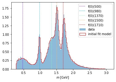
optimized_parameters = fit_result["parameter_values"]
intensity.update_parameters(optimized_parameters)
compare_model("m_12", data_set, phsp_set, intensity)
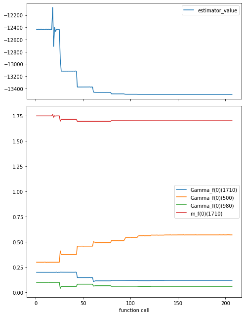
fit_traceback = pd.read_csv("traceback.csv")
fig, (ax1, ax2) = plt.subplots(
    2, figsize=(7, 9), sharex=True, gridspec_kw={"height_ratios": [1, 2]}
)
fit_traceback.plot("function_call", "estimator_value", ax=ax1)
fit_traceback.plot("function_call", sorted(initial_parameters), ax=ax2)
fig.tight_layout()
ax2.set_xlabel("function call");
Step-by-step workflow
The following pages go through the usual workflow when using tensorwaves. The output in each of these steps is written to disk, so that each notebook can be run separately.