Step 3: Perform fit
As explained in the previous step, a Model object and its lambdified Function form behave just like a mathematical function that takes a set of data points as an argument and returns a list of intensities (real numbers). At this stage, we want to optimize the parameters of the intensity model, so that it matches the distribution of our data sample. This is what we call ‘performing a fit’.
First, load the relevant data from the previous steps.
import pickle

from tensorwaves.model import SympyModel

with open("helicity_model.pickle", "rb") as stream:
    model = pickle.load(stream)
with open("data_set.pickle", "rb") as stream:
    data_set = pickle.load(stream)
with open("phsp_set.pickle", "rb") as stream:
    phsp_set = pickle.load(stream)
sympy_model = SympyModel(
    expression=model.expression,
    parameters=model.parameters,
)
3.1 Define estimator
To perform a fit, you need to define an Estimator. An estimator is a measure for the discrepancy between the intensity model and the data distribution to which you fit. In PWA, we usually use an unbinned negative log likelihood estimator.
Generally, the intensity model is not normalized, but a log likelihood estimator requires a normalized function. This is where the phase space dataset comes into play again: the intensity is evaluated separately with the phase space dataset so that the output of the Function can be normalized with it. The phase space sample is therefore a required argument!
from tensorwaves.estimator import UnbinnedNLL

estimator = UnbinnedNLL(
    sympy_model,
    data_set,
    phsp_set,
    backend="jax",
)
Note that the UnbinnedNLL can be expressed with different backends (it creates a LambdifiedFunction internally from the template Model). Here, we use jax, which is turns out to be the fastest backend for this model.
3.2 Optimize intensity model
Specify fit parameters
Starting the fit itself is quite simple: just create an optimizer instance of your choice, here Minuit2, and call its optimize() method to start the fitting process. The optimize() method requires a mapping of parameter names to their initial values. Only the parameters listed in the mapping are optimized.
Let’s first select a few of the parameters that we saw in Step 3.1 and feed them to the optimizer to run the fit. Notice that we modify the parameters slightly to make the fit more interesting (we are running fitting to a data sample that was generated with this very same amplitude model after all).
initial_parameters = {
    "C[J/\\psi(1S) \\to f_{0}(1500)_{0} \\gamma_{+1};f_{0}(1500) \\to \\pi^{0}_{0} \\pi^{0}_{0}]": 1.0
    + 0.0j,
    "Gamma_f(0)(500)": 0.3,
    "Gamma_f(0)(980)": 0.1,
    "m_f(0)(1710)": 1.75,
    "Gamma_f(0)(1710)": 0.2,
}
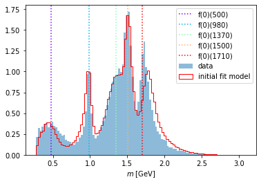
Recall that a Function object computes the intensity for a certain dataset. This can be seen now nicely when we use these intensities as weights on the phase space sample and plot it together with the original dataset. Here, we look at the invariant mass distribution projection of the final states 1 and 2, which, as we saw before, are the final state particles \(\pi^0,\pi^0\).
Don’t forget to use update_parameters() first!
import matplotlib.pyplot as plt
import numpy as np
from matplotlib import cm

reaction_info = model.adapter.reaction_info
intermediate_states = sorted(
    (
        p
        for p in model.particles
        if p not in reaction_info.final_state.values()
        and p not in reaction_info.initial_state.values()
    ),
    key=lambda p: p.mass,
)

evenly_spaced_interval = np.linspace(0, 1, len(intermediate_states))
colors = [cm.rainbow(x) for x in evenly_spaced_interval]


def indicate_masses():
    plt.xlabel("$m$ [GeV]")
    for i, p in enumerate(intermediate_states):
        plt.gca().axvline(
            x=p.mass, linestyle="dotted", label=p.name, color=colors[i]
        )


def compare_model(
    variable_name,
    data_set,
    phsp_set,
    intensity_model,
    bins=100,
):
    data = data_set[variable_name]
    phsp = phsp_set[variable_name]
    intensities = intensity_model(phsp_set)
    axis = plt.gca()
    axis.hist(data, bins=bins, alpha=0.5, label="data", density=True)
    axis.hist(
        phsp,
        weights=intensities,
        bins=bins,
        histtype="step",
        color="red",
        label="initial fit model",
        density=True,
    )
    indicate_masses()
    plt.legend()
from tensorwaves.model import LambdifiedFunction

intensity = LambdifiedFunction(sympy_model, backend="numpy")
intensity.update_parameters(initial_parameters)
compare_model("m_12", data_set, phsp_set, intensity)
Custom callbacks
The Minuit2 class allows one to insert certain callbacks. Callbacks are used to insert behavior into the Optimizer.optimize() method. The callbacks module provides several handy callback classes, but it’s also possible to define custom callbacks into the Optimizer by defining a custom Callback class. Here’s one that live updates a plot of the latest fit model!
import os

from IPython.display import clear_output
from tensorwaves.optimizer.callbacks import Callback

variable_to_plot = "m_12"
is_doc = "READTHEDOCS" in os.environ or "EXECUTE_NB" in os.environ


class PyplotCallback(Callback):
    def __init__(self, step_size=10):
        self.__step_size = step_size
        self.__fig = None
        self.__ax = None
        self.__latest_parameters = {}

    def on_iteration_end(self, function_call, logs=None):
        self.__latest_parameters = logs["parameters"]
        if is_doc:
            return
        if function_call % self.__step_size != 0:
            return
        if function_call > 75:
            return
        self.update_plot(nbins=80)
        clear_output(wait=True)
        display(plt.gcf())

    def on_function_call_end(self):
        self.update_plot(nbins=200)

    def update_plot(self, nbins: int):
        if self.__fig is None or self.__ax is None:
            self.__fig, self.__ax = plt.subplots(1, figsize=(8, 5))
        data = data_set[variable_to_plot]
        phsp = phsp_set[variable_to_plot]
        intensity.update_parameters(self.__latest_parameters)
        intensities = intensity(phsp_set)
        self.__ax.cla()
        self.__ax.hist(data, bins=nbins, alpha=0.5, label="data", density=True)
        self.__ax.hist(
            phsp,
            weights=intensities,
            bins=nbins,
            histtype="step",
            color="red",
            label="fit model",
            density=True,
        )
        self.__ax.set_xlim((0.25, 2.5))
        self.__ax.set_ylim((0, 1.9))
        indicate_masses()
        plt.gcf().legend()
In the fit example below, we want to use several callbacks together. To do so, we ‘stack’ them together with CallbackList:
from tensorwaves.optimizer.callbacks import (
    CallbackList,
    CSVSummary,
    TFSummary,
    YAMLSummary,
)

callbacks = CallbackList(
    [
        CSVSummary("fit_traceback.csv", step_size=2),
        PyplotCallback(),  # comment this line for raw fit performance
        TFSummary(),
        YAMLSummary("current_fit_result.yaml"),
    ]
)
Perform fit
Finally, we create an Optimizer to optimize() the model (which is embedded in the Estimator). Here, we choose the Minuit2 optimizer, which is the most common optimizer in high-energy physics. Since we constructed the UnbinnedNLL with jax, can an optimize the model with analytic gradient over the LambdifiedFunction:
from tensorwaves.optimizer.minuit import Minuit2

minuit2 = Minuit2(
    callback=callbacks,
    use_analytic_gradient=False,
)
result = minuit2.optimize(estimator, initial_parameters)
result
{'minimum_valid': True,
 'parameter_values': {'Gamma_f(0)(500)': 0.5451752218891177,
  'Gamma_f(0)(980)': 0.060940067974818865,
  'm_f(0)(1710)': 1.7035573371314008,
  'Gamma_f(0)(1710)': 0.12243585272818946,
  'C[J/\\psi(1S) \\to f_{0}(1500)_{0} \\gamma_{+1};f_{0}(1500) \\to \\pi^{0}_{0} \\pi^{0}_{0}]': (0.9997333125682356+0.04579068575933221j)},
 'parameter_errors': {'Gamma_f(0)(500)': 0.013932761082030364,
  'Gamma_f(0)(980)': 0.0017551972931582715,
  'm_f(0)(1710)': 0.001270929385015649,
  'Gamma_f(0)(1710)': 0.003616781026129371,
  'C[J/\\psi(1S) \\to f_{0}(1500)_{0} \\gamma_{+1};f_{0}(1500) \\to \\pi^{0}_{0} \\pi^{0}_{0}]': (0.017483571175615806+0.02299354970835373j)},
 'log_likelihood': -15613.190099057005,
 'function_calls': 207,
 'execution_time': 35.89210796356201}
As can be seen, the values of the optimized parameters in the result are again comparable to the original values that are contained in the model (SympyModel.parameters):
optimized_parameters = result["parameter_values"]
for p in optimized_parameters:
    print(p)
    print(f"  initial:   {initial_parameters[p]:.3}")
    print(f"  optimized: {optimized_parameters[p]:.3}")
    print(f"  original:  {sympy_model.parameters[p]:.3}")
Gamma_f(0)(500)
  initial:   0.3
  optimized: 0.545
  original:  0.55
Gamma_f(0)(980)
  initial:   0.1
  optimized: 0.0609
  original:  0.06
m_f(0)(1710)
  initial:   1.75
  optimized: 1.7
  original:  1.7
Gamma_f(0)(1710)
  initial:   0.2
  optimized: 0.122
  original:  0.123
C[J/\psi(1S) \to f_{0}(1500)_{0} \gamma_{+1};f_{0}(1500) \to \pi^{0}_{0} \pi^{0}_{0}]
  initial:   (1+0j)
  optimized: (1+0.0458j)
  original:  (1+0j)
3.3 Export and import
In 3.2 Optimize intensity model, we initialized Minuit2 with some callbacks that are Loadable. Such callback classes offer the possibility to Loadable.load_latest_parameters(), so you can pick up the optimize process in case it crashes or if you pause it. Loading the latest parameters goes as follows:
latest_parameters = YAMLSummary.load_latest_parameters(
    "current_fit_result.yaml"
)
latest_parameters
{'Gamma_f(0)(500)': 0.5451752218891177,
 'Gamma_f(0)(980)': 0.060940067974818865,
 'm_f(0)(1710)': 1.7036584692982328,
 'Gamma_f(0)(1710)': 0.12243585272818946,
 'C[J/\\psi(1S) \\to f_{0}(1500)_{0} \\gamma_{+1};f_{0}(1500) \\to \\pi^{0}_{0} \\pi^{0}_{0}]': (0.9997333125682356+0.04747216966054012j)}
To restart the fit with the latest parameters, simply rerun as before.
minuit2 = Minuit2()
minuit2.optimize(estimator, latest_parameters)
{'minimum_valid': True,
 'parameter_values': {'Gamma_f(0)(500)': 0.5451861055908453,
  'Gamma_f(0)(980)': 0.060944000346352216,
  'm_f(0)(1710)': 1.7035525248740562,
  'Gamma_f(0)(1710)': 0.12244306481714447,
  'C[J/\\psi(1S) \\to f_{0}(1500)_{0} \\gamma_{+1};f_{0}(1500) \\to \\pi^{0}_{0} \\pi^{0}_{0}]': (0.9997164353449564+0.045915633065424476j)},
 'parameter_errors': {'Gamma_f(0)(500)': 0.013933166182520463,
  'Gamma_f(0)(980)': 0.0017553686440790364,
  'm_f(0)(1710)': 0.0012709928980932875,
  'Gamma_f(0)(1710)': 0.0036170387263838636,
  'C[J/\\psi(1S) \\to f_{0}(1500)_{0} \\gamma_{+1};f_{0}(1500) \\to \\pi^{0}_{0} \\pi^{0}_{0}]': (0.017483891718730354+0.022994719653933494j)},
 'log_likelihood': -15613.190083634834,
 'function_calls': 97,
 'execution_time': 15.706201314926147}
Lo and behold: the parameters were already optimized, so the fit converged faster!
3.4 Visualize
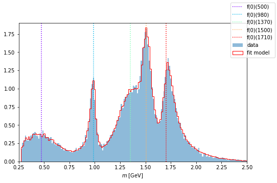
Plot optimized model
Using the same method as above, we renew the parameters of the Function and plot it again over the data distribution.
intensity.update_parameters(latest_parameters)
compare_model("m_12", data_set, phsp_set, intensity)

Analyze optimization process
Note that in Step 3.2, we initialized Minuit2 with a TFSummary callback as well. Its output files provide a nice, interactive representation of the fit process and can be viewed with TensorBoard as follows:
tensorboard --logdir logs
import tensorboard as tb

tb.notebook.list()  # View open TensorBoard instances
tb.notebook.start(args_string="--logdir logs")
See more info here
%load_ext tensorboard
%tensorboard --logdir logs
See more info here
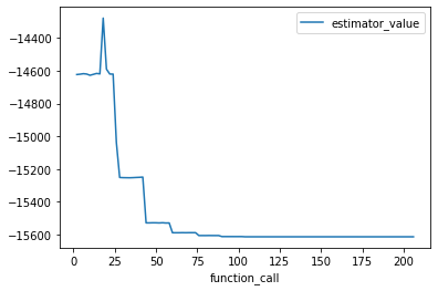
An alternative would be to use the output of the CSVSummary callback. Here’s an example:
import pandas as pd
fit_traceback = pd.read_csv("fit_traceback.csv")
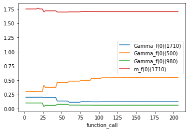
fit_traceback.plot("function_call", "estimator_value")
fit_traceback.plot("function_call", sorted(initial_parameters));