Unbinned fit

Imagine we have the following data distribution over \(x,y\):

import numpy as np

sample_size = 50_000
rng = np.random.default_rng(seed=0)
data = {
    "x": rng.rayleigh(size=sample_size),
    "y": rng.normal(size=sample_size),
}

Show code cell source Hide code cell source

%config InlineBackend.figure_formats = ['png']
import matplotlib as mpl
import matplotlib.pyplot as plt
from matplotlib import cm

mpl.rcParams["figure.dpi"] = 300

fig, ((ax_x, empty), (ax2d, ax_y)) = plt.subplots(
    ncols=2,
    nrows=2,
    figsize=(8, 5),
    gridspec_kw=dict(
        height_ratios=[1, 5],
        width_ratios=[7, 1],
    ),
)
fig.subplots_adjust(wspace=0, hspace=0)
empty.remove()
ax2d.set_xlabel("$x$")
ax2d.set_ylabel("$y$")
ax2d.get_shared_x_axes().join(ax2d, ax_x)
ax2d.get_shared_y_axes().join(ax2d, ax_y)
for ax in [ax_x, ax_y]:
    ax.set_xticks([])
    ax.set_yticks([])
    for side in ["top", "right", "bottom", "left"]:
        ax.spines[side].set_visible(False)

bins_x, bins_y = 80, 50
bin_values, bin_edges_x, bin_edges_y, _ = ax2d.hist2d(
    data["x"], data["y"], bins=(bins_x, bins_y), cmap=cm.coolwarm
)
xlim = 0, 4
ylim = -3, +3
ax2d.set_xlim(*xlim)
ax2d.set_ylim(*ylim)
ax_x.fill_between(
    x=(bin_edges_x[1:] + bin_edges_x[:-1]) / 2,
    y1=np.sum(bin_values, axis=1),
    step="pre",
    alpha=0.6,
)
ax_y.fill_between(
    x=np.sum(bin_values, axis=0),
    y1=(bin_edges_y[1:] + bin_edges_y[:-1]) / 2,
    step="pre",
    alpha=0.6,
)
plt.show()

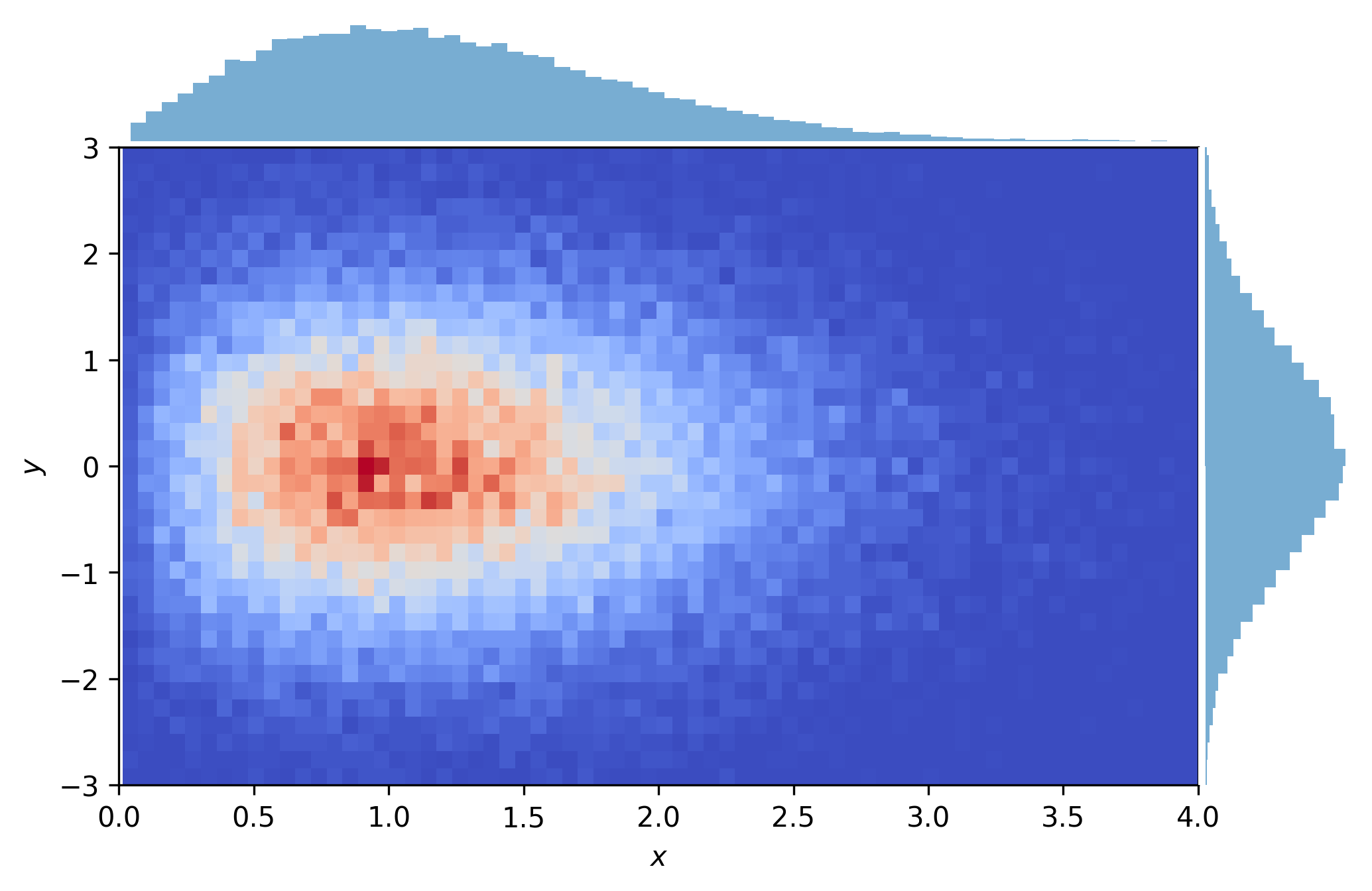
The data distribution has been generated by numpy.random.normal() and numpy.random.rayleigh() and can therefore be described by the following expression:

import sympy as sp


def rayleigh(x, sigma):
    return x / sigma**2 * sp.exp(-(x**2) / (2 * sigma**2))


def gaussian(x, mu, sigma):
    return sp.exp(-((x - mu) ** 2) / (2 * sigma**2)) / sp.sqrt(
        2 * sp.pi * sigma**2
    )


x, y, mu, sigma_x, sigma_y = sp.symbols("x y mu sigma_x sigma_y")
expression = rayleigh(x, sigma_x) * gaussian(y, mu, sigma_y)
expression

\[\displaystyle \frac{\sqrt{2} x e^{- \frac{x^{2}}{2 \sigma_{x}^{2}}} e^{- \frac{\left(- \mu + y\right)^{2}}{2 \sigma_{y}^{2}}}}{2 \sqrt{\pi} \sigma_{x}^{2} \sqrt{\sigma_{y}^{2}}}\]

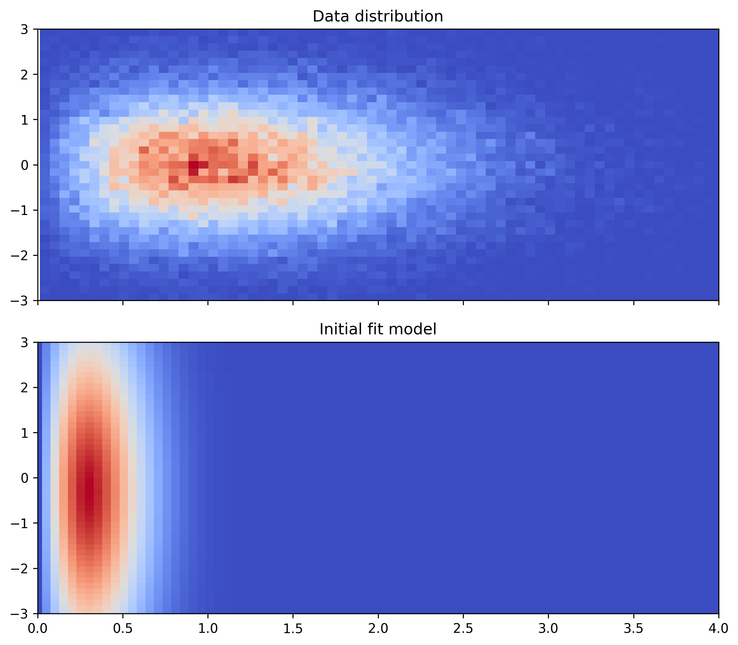
We would like to find values for \(\mu, \sigma_x, \sigma_y\), so that the expression describe this distribution as best as possible. For this, we first formulate this expression as a ParametrizedFunction in a specific computational backend, so that we can use it to quickly compute values over a number of data points. We also provide some initial guesses for the parameter values:

from tensorwaves.function.sympy import create_parametrized_function

function = create_parametrized_function(
    expression,
    parameters={mu: -0.3, sigma_x: 0.3, sigma_y: 2.7},
    backend="jax",
)
initial_parameters = function.parameters

The function can be used to visualize the expression with this choice of parameter values over a certain \(xy\)-domain and compare it to the original data distribution.

Show code cell source Hide code cell source

X = np.linspace(*xlim, bins_x)
Y = np.linspace(*ylim, bins_y)
X, Y = np.meshgrid(X, Y)

function.update_parameters(initial_parameters)
Z = function({"x": X, "y": Y})

fig, (ax1, ax2) = plt.subplots(
    nrows=2, sharex=True, figsize=(8, 7), tight_layout=True
)
ax1.set_title("Data distribution")
ax2.set_title("Initial fit model")
ax1.hist2d(data["x"], data["y"], cmap=cm.coolwarm, bins=(bins_x, bins_y))
ax2.pcolormesh(X, Y, Z, cmap=cm.coolwarm)
for ax in [ax1, ax2]:
    ax.set_xlim(*xlim)
    ax.set_ylim(*ylim)
plt.show()

Next, we use a UnbinnedNLL optimize the parameters with regard to the data distribution. Note that a UnbinnedNLL requires a domain over which to integrate the ParametrizedFunction, in order to normalize the log likelihood.

from tensorwaves.estimator import UnbinnedNLL
from tensorwaves.optimizer import Minuit2

integration_domain = {
    "x": rng.uniform(0, 4, size=200_000),
    "y": rng.uniform(-3, +3, size=200_000),
}
estimator = UnbinnedNLL(function, data, integration_domain, backend="jax")
optimizer = Minuit2()
fit_result = optimizer.optimize(estimator, initial_parameters)
fit_result

FitResult(
 minimum_valid=True,
 execution_time=1.5926756858825684,
 function_calls=262,
 estimator_value=-41104.124054898595,
 parameter_values={
  'mu': -0.0033345752250491132,
  'sigma_x': 1.0015388337105258,
  'sigma_y': 1.0094470816077672,
 },
 parameter_errors={
  'mu': 0.004564636117794515,
  'sigma_x': 0.0022676214391666658,
  'sigma_y': 0.0034326511736429426,
 },
)

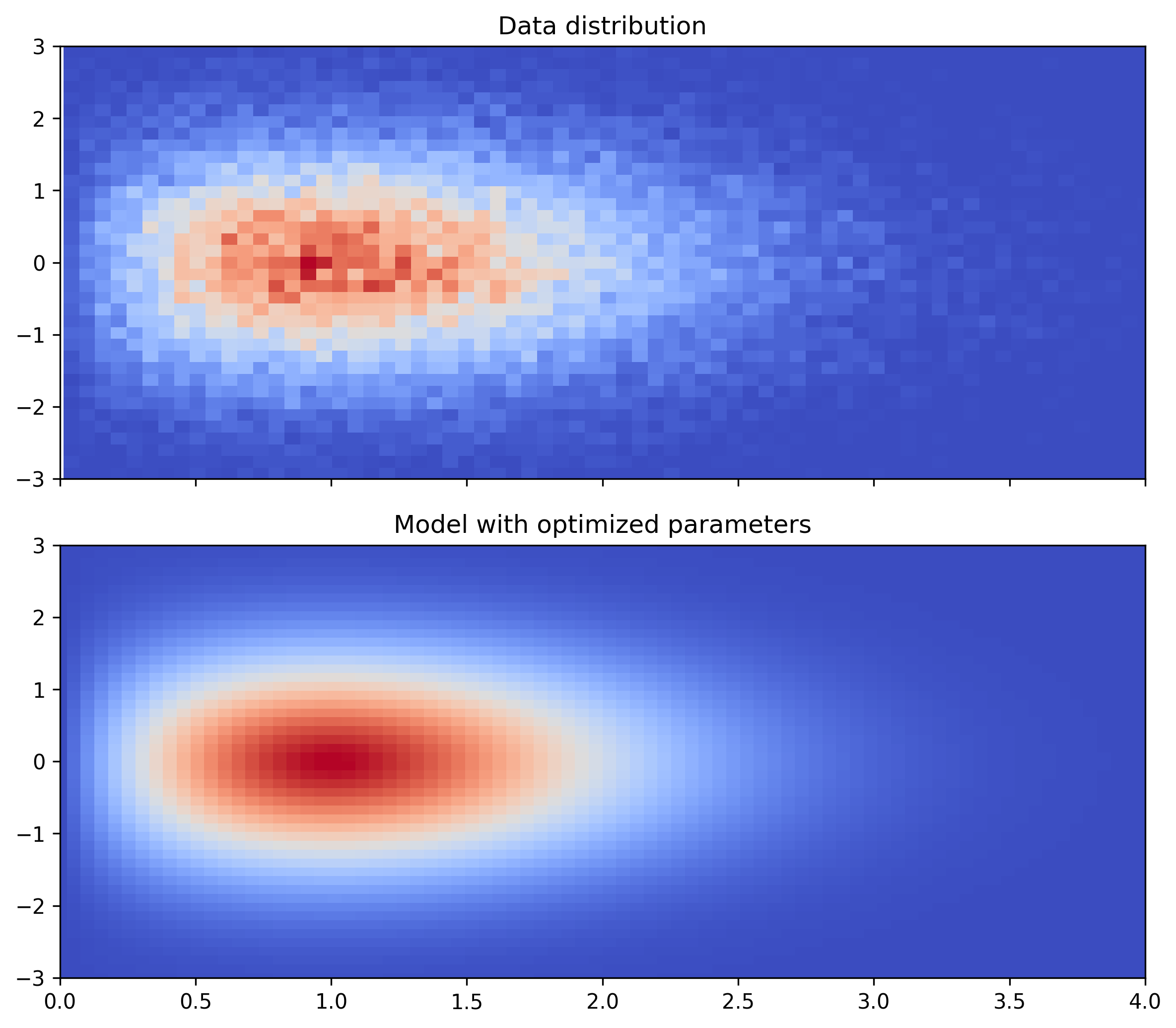
The values are indeed close to the default values for numpy.random.rayleigh() (\(\sigma_x=1\)) numpy.random.normal() (\(\mu=0, \sigma_y=1\)), with which the data distribution was generated.

Show code cell source Hide code cell source

function.update_parameters(fit_result.parameter_values)
Z = function({"x": X, "y": Y})

fig, (ax1, ax2) = plt.subplots(
    nrows=2, sharex=True, figsize=(8, 7), tight_layout=True
)
ax1.set_title("Data distribution")
ax2.set_title("Model with optimized parameters")
ax1.hist2d(data["x"], data["y"], cmap=cm.coolwarm, bins=(bins_x, bins_y))
ax2.pcolormesh(X, Y, Z, cmap=cm.coolwarm)
for ax in [ax1, ax2]:
    ax.set_xlim(*xlim)
    ax.set_ylim(*ylim)
plt.show()